Spherical Harmonic Basis Functions Part 1

Real spherical harmonic basis functions, rows represents the degree, columns the order. Represented in spherical coordinates where the radius is the basis function value.

$~$

$~$

Disclaimer: The following proofs are not rigorous and skip over important steps to make the post easier to read. Full proofs can be found online.

Table of Contents

1. Summary
2. Definition
3. Properties
   1. Orthogonality
   2. Expansion
4. Complex and Real Forms
5. Visualizations
6. Tables
   1. Associated Legendre Polynomials
   2. Complex Spherical Harmonics
   3. Real Spherical Harmonics

Summary

This is part 1 in a series about spherical harmonics and their uses in rendering. This post will focus on the definition and properties of spherical harmonic basis functions. We will define a normalized version of spherical harmonics, show they form a basis and establish that they can approximate functions over the sphere.

Definition

By solving Laplace’s equation we found that the angular part is:

\[Y_{\ell}^{m}(\theta, \varphi) = P_\ell^m(\cos\theta)e^{im\varphi}\]

Where $\ell, m$ are integers, $\ell\geq 0$ and $-\ell \leq m \leq \ell$ and $P_{\ell}^{m}$ is the associated Legendre polynomial. $\ell$ is called the degree (also bands) and $m$ the order of the spherical harmonic $Y_\ell^m$. We will not be directly using the solution above as it lacks a normalizing constant. To arrive at the final definition, we need to normalze $Y_{\ell}^{m}(\theta, \varphi)$. Using the $L_2$ inner product, it’s possible to show that:

\[\langle Y_{\ell}^{m},Y_{\ell}^{m} \rangle = \int_{0}^{2\pi} \int_{0}^{\pi} Y_{\ell}^{m} (\theta, \varphi)^2 \sin \theta d\theta d\varphi = \frac{4\pi}{2\ell + 1} \frac{(\ell + m)!}{(\ell - m)!}\]

Proving the statement above requires the inner product of the complex exponential and associated Legendre polynomial. When taking the square root we get the norm:

\[|| Y_{\ell}^{m} || = \sqrt{ \frac{4\pi}{2\ell + 1} \frac{(\ell + m)!}{(\ell - m)!}}\]

Now that we have the norm, let’s define $Y_{\ell}^{m}$ as:

\[Y_{\ell}^{m}(\theta, \varphi) = (-1)^{m} \sqrt{ \frac{2\ell + 1}{4\pi} \frac{(\ell - m)!}{(\ell + m) }} P_\ell^m(\cos\theta)e^{im\varphi}\]

The term $(-1)^{m}$ is called Condon-Shortley phase and is used by convention in physics to simplify some equations. This definition is valid for $\ell \geq 0$, $-\ell \leq m \leq \ell$, having a special case for negative $m$ values:

\[Y_{\ell}^{-m}(\theta, \varphi) = (-1)^m (Y_{\ell}^{m}(\theta, \varphi))^*\]

This can be shown using this equation from the associated Legendre polynomials:

\[P_\ell^{-m}(x) = (-1)^m \frac{(\ell-m)!}{(\ell+m)!}P_\ell^m(x)\]

And the facts that the complex conjugate of real functions is identity and $(e^{im\varphi})^* = e^{-im\varphi}$.

Properties

Orthogonality

For fixed $m$, with the $L_2$ inner product we have:

\[\langle Y_{\ell}^{m},Y_{\ell'}^{m} \rangle = \int_{0}^{2\pi} \int_{0}^{\pi} Y_{\ell}^{m} (\theta, \varphi) Y_{\ell'}^{m} (\theta, \varphi) \sin \theta d\theta d\varphi = \delta_{\ell \ell'}\]

Where $\delta_{\ell \ell’}$ is the Kronecker delta function, being 0 when $\ell \neq \ell’$ and 1 when $\ell = \ell’$. and relies on the orthogonality of the Legendre polynomials and the complex exponential. When $\ell = \ell’$ we get back the inner product which is 1 after normalizing the spherical harmonics definition.

If we consider the case when $m$ is not fixed, we can show that the complex exponential is orthogonal (using the complex version of the $L_2$ inner product):

\[\int_{0}^{2\pi} (e^{im\varphi})^*e^{im'\varphi} d\varphi = 2\pi \delta_{m m'}\]

When $m=m’$, the numerator vanishes and the result is $2\pi$, otherwise it cancels out to 0. Combining this with the previous result we get the orthogonality for both $m$ and $\ell$:

\[\langle Y_{\ell}^{m},Y_{\ell'}^{m'} \rangle = \int_{0}^{2\pi} \int_{0}^{\pi} Y_{\ell}^{m} (\theta, \varphi) Y_{\ell'}^{m'} (\theta, \varphi) \sin \theta d\theta d\varphi = \delta_{\ell \ell'} \delta_{m m'}\]

Since the norm of $Y_{\ell}^{m}$ is 1, they are also orthonormal. A more rigorous proof of orthogonality can be found here.

Expansion

Since $Y_\ell^m$ forms a set of orthonormal functions, they can be used to expand functions as a linear combination of spherical harmonics as follows:

\[f(\theta, \varphi) = \sum_{\ell = 0}^{\infty} \sum_{m=-\ell}^{\ell} f_\ell^m Y_\ell^m(\theta, \varphi)\]

Where $f_\ell^m \in \mathbb{C}$ are the basis function coefficients. This holds for functions $f$ that are square-integrable on $S^2$, meaning that the integral of $\lvert f^2 \rvert$ is finite. The coefficients can be found by integrating the product of the complex conjugate of $Y_\ell^m$ and $f$ over the sphere. The Wikipedia entry for spherical harmonics has more details on how it works.

This expansion property also holds for real spherical harmonics, and it guarantees that the coefficients $f_\ell^m$ are in $\mathbb{R}$ instead of $\mathbb{C}$.

There are many more properties (eg. rotation, parity) about spherical harmonics and I will try to explore them in details in future posts

$~$

Complex and Real Forms

The definition of the spherical harmonics above is from the surface of the sphere to the complex numbers:

\[Y_{\ell}^{m}: S^2 \rightarrow \mathbb{C}\]

Where $S^2$ is the surface of the sphere defined with $\theta\in [0, \pi]$ and $\varphi \in [0, 2\pi]$. If we want to map to the real numbers, we need an different definition. Let $Y_{\ell m}: S^2 \rightarrow \mathbb{R}$ be the real spherical harmonics with the following definition:

\[Y_{\ell m} = \begin{cases} \frac{i}{\sqrt{2}}\left( Y_{\ell}^{m} - (-1)^m Y_{\ell}^{-m} \right), & \mbox{if } m < 0 \\ Y_{\ell}^{0}, & \mbox{if } m = 0 \\ \frac{i}{\sqrt{2}}\left( Y_{\ell}^{-m} + (-1)^m Y_{\ell}^{m} \right), & \mbox{if } m > 0 \end{cases}\]

We can expand this definition in terms of the associated Legendre polynomials and trigonometric functions.

\[Y_{\ell m} = \begin{cases} \sqrt{2} \sqrt{\frac{2\ell + 1}{4 \pi} \frac{ (\ell - |m|)!}{(\ell + |m|)!}} P_{\ell}^{|m|} (\cos \theta) \sin (|m|\varphi), & \mbox{if } m < 0 \\ Y_{\ell}^{0}, & \mbox{if } m = 0 \\ \sqrt{2} \sqrt{\frac{2\ell + 1}{4 \pi} \frac{ (\ell - m)!}{(\ell + m)!}} P_{\ell}^{m} (\cos \theta) \cos (m\varphi), & \mbox{if } m > 0 \end{cases}\]

These can be found by using the identity for negative $m$ values, then rewriting the equations in terms of the associated Legendre polynomials. Real spherical harmonics also form an orthonormal basis and share many other properties with complex spherical harmonics.

Visualizations

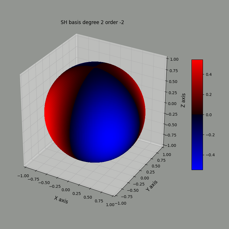
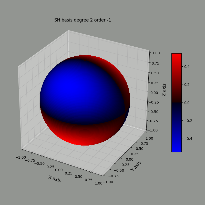
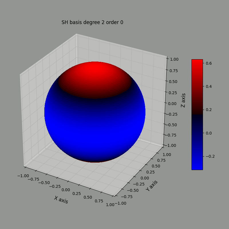
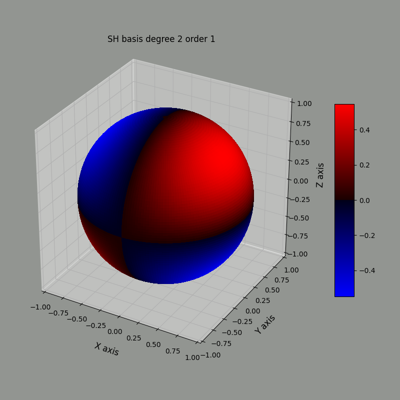
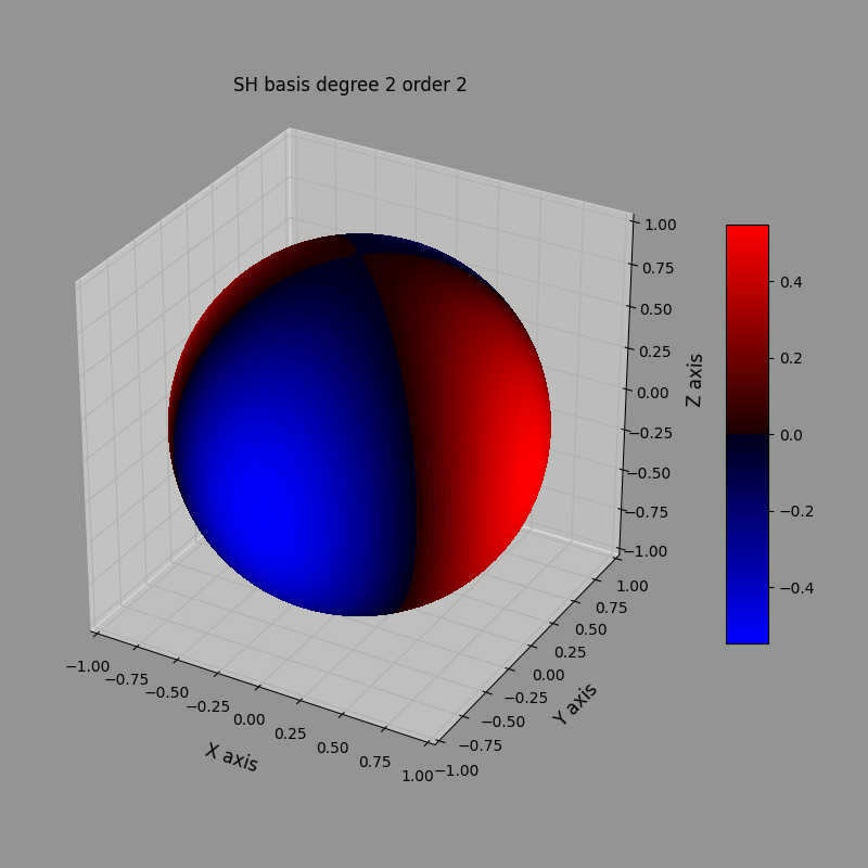
There are 2 main ways to represent real spherical harmonics in 3D. One is to use a heat map where the color represents the basis function value at a specific point on the sphere and the other is using the basis function value as the radius in spherical coordinates.

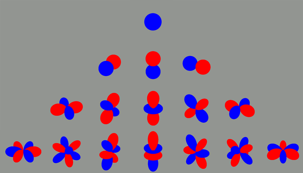
The images below represent the $\ell=2$ basis functions, with $m=-2\ldots2$ from left to right using the heat map method. Red is positive, blue is negative.

Using the radius method, we can represent the same basis functions this way:

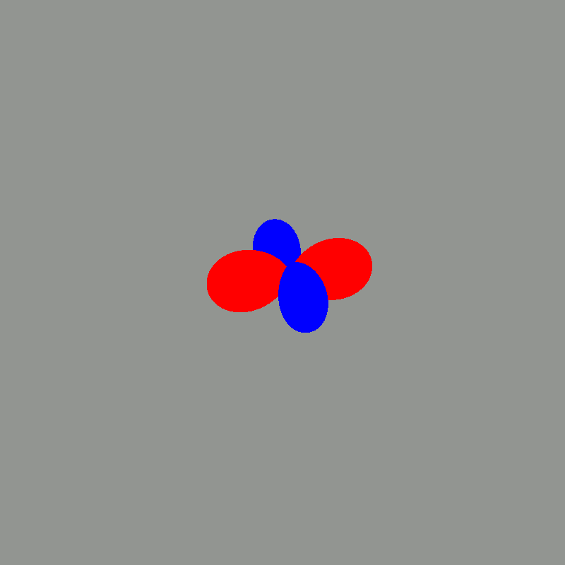
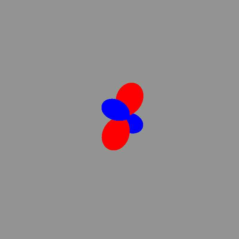
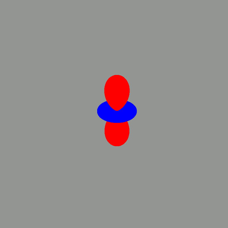
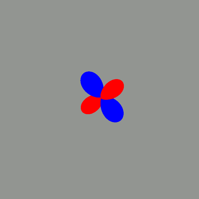
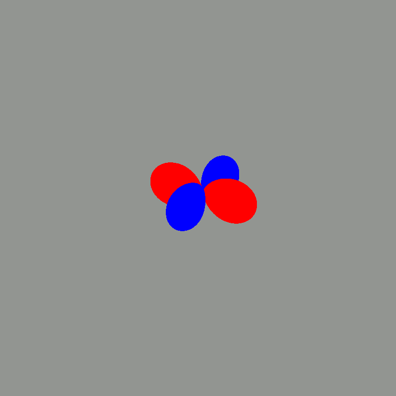
Notice that the blue and red regions match between both representation.

To generate these images, I wrote some code to evaluate real spherical harmonics using a set of points on the sphere. The entire source code can be found in this GitHub repository and is written in Python. It supports up to $\ell=3$. It also contains Maple code which implements the associated Legendre polynomials, complex and real spherical harmonics to verify that the results match existing spherical harmonics tables.

Tables

Depending on the definition of Legendre polynomials and spherical harmonics, the basis functions might change somewhat. I will rely on the definitions used in the current and previous posts to compute the spherical harmonic basis functions.

The final equations will be in terms of cartesian coordinates $x, y, z$. To convert from spherical to cartesian coordinates we need these equations:

\[\begin{align} x &= r\sin\theta\cos\varphi \\ y &= r\sin\theta\sin\varphi \\ z &= r\cos\theta \end{align}\]

Associated Legendre Polynomial

\[\begin{align} P_{0}^{ 0} &= 1 \\ \\ P_{1}^{-1} &= -\frac{1}{2}\sqrt{1 - x^2} \\ P_{1}^{ 0} &= x \\ P_{1}^{ 1} &= \sqrt{1 - x^2} \\ \\ P_{2}^{-2} &= \frac{1}{8}(1-x^2) \\ P_{2}^{-1} &= -\frac{x}{2}\sqrt{1 - x^2} \\ P_{2}^{ 0} &= \frac{1}{2}(3x^2 -1) \\ P_{2}^{ 1} &= 3x\sqrt{x^2 - 1} \\ P_{2}^{ 2} &= 3(1-x^2) \end{align}\]

Complex Spherical Harmonics

\[\begin{align} Y_{0}^{ 0} &= \frac{1}{2}\sqrt{\frac{1}{\pi}} \\ \\ Y_{1}^{-1} &= \frac{1}{2}\sqrt{\frac{3}{2\pi}} \frac{(x-iy)}{r} \\ Y_{1}^{ 0} &= \frac{1}{2}\sqrt{\frac{3}{\pi}} \frac{z}{r} \\ Y_{1}^{ 1} &= -\frac{1}{2}\sqrt{\frac{3}{2\pi}} \frac{(x+iy)}{r} \\ \\ Y_{2}^{-2} &= \frac{1}{4}\sqrt{\frac{15}{2\pi}}\frac{(x-iy)^2}{r^2} \\ Y_{2}^{-1} &= \frac{1}{2}\sqrt{\frac{15}{2\pi}}\frac{z(x-iy)}{r^2} \\ Y_{2}^{ 0} &= \frac{1}{4}\sqrt{\frac{5}{\pi}}\frac{(2z^2-x^2-y^2)}{r^2} \\ Y_{2}^{ 1} &= -\frac{1}{2}\sqrt{\frac{15}{2\pi}}\frac{z(x+iy)}{r^2} \\ Y_{2}^{ 2} &= \frac{1}{4}\sqrt{\frac{15}{2\pi}}\frac{(x+iy)^2}{r^2} \end{align}\]

Real Spherical Harmonics

\[\begin{align} Y_{0,0} &= \frac{1}{2}\sqrt{\frac{1}{\pi}} \\ \\ Y_{1,-1} &= \sqrt{\frac{3}{4\pi}} \frac{y}{r} \\ Y_{1, 0} &= \sqrt{\frac{3}{4\pi}} \frac{z}{r} \\ Y_{1, 1} &= \sqrt{\frac{3}{4\pi}} \frac{x}{r} \\ \\ Y_{2,-2} &= \frac{1}{2}\sqrt{\frac{15}{\pi}}\frac{xy}{r^2} \\ Y_{2,-1} &= \frac{1}{2}\sqrt{\frac{15}{\pi}}\frac{yz}{r^2} \\ Y_{2, 0} &= \frac{1}{4}\sqrt{\frac{5}{\pi}}\frac{(2z^2-x^2-y^2)}{r^2} \\ Y_{2, 1} &= \frac{1}{2}\sqrt{\frac{15}{\pi}}\frac{xz}{r^2} \\ Y_{2, 2} &= \frac{1}{4}\sqrt{\frac{15}{\pi}}\frac{(x^2-y^2)}{r^2} \end{align}\]

References

• https://en.wikipedia.org/wiki/Spherical_harmonics
• https://www.physics.uoguelph.ca/chapter-3-legendre-polynomials
• https://www.physics.uoguelph.ca/chapter-4-spherical-harmonics
• https://en.wikipedia.org/wiki/Table_of_spherical_harmonics
• https://github.com/Beatthezombie/SphericalHarmonicsFromScratch

Comments

This comment section uses GitHub issues. Join the discussion for this post on this issue.